INDEX MATCH in Excel: The Lookup That Works in Every Version

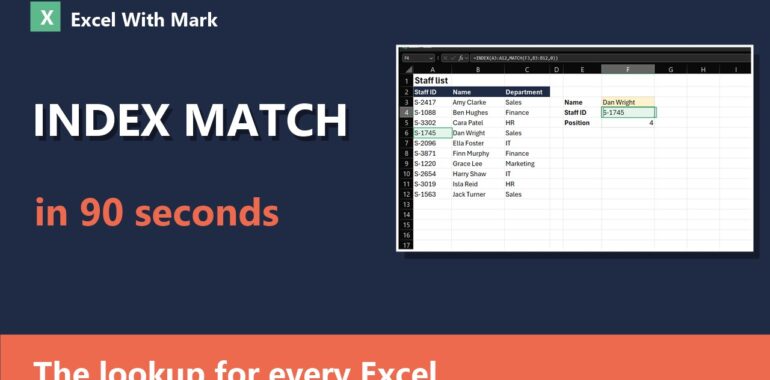
If you’ve ever been stuck because VLOOKUP can’t look to the left, or you’ve sent a spreadsheet to someone on an older version of Excel and XLOOKUP turned into #NAME?, INDEX MATCH is the answer. It works in every version of Excel, it doesn’t care which side your answer column is on, and once you’ve seen it broken into two parts it’s easy.

Here’s the whole thing in 90 seconds:

The example: find a staff ID from a name

We have a staff list with Staff ID in column A, Name in column B and Department in column C. We want to type a name in F3 and get that person’s staff ID back. The ID is to the left of the name, so VLOOKUP can’t do it.

Step 1: MATCH finds the position

MATCH tells you where something is in a list. In F5, type:

=MATCH(F3,B3:B12,0)

• F3 is what to find (the name).
• B3:B12 is where to find it (the name column).
• 0 means an exact match. Always use 0 for lookups like this.

For “Dan Wright” it returns 4, because Dan is the fourth name in the list.

Step 2: INDEX brings back the value

INDEX does the opposite: give it a column and a position, and it hands back whatever is in that spot. =INDEX(A3:A12,4) returns the 4th staff ID.

Now swap the 4 for the MATCH formula, and you have INDEX MATCH:

=INDEX(A3:A12,MATCH(F3,B3:B12,0))

Read it as: “bring back the staff ID from the row where the name matches F3.” Change the name in F3 and the ID updates straight away.

Why use INDEX MATCH instead of VLOOKUP?

• It can look left. The answer column can be anywhere.
• It doesn’t break when you insert columns. VLOOKUP’s column number (the 3 in VLOOKUP(F3,A:C,3,FALSE)) points at the wrong column if someone inserts one. INDEX MATCH points at the actual columns.
• It works in every version of Excel, including Excel 2010, 2013, 2016, 2019, Excel for Mac and Excel for the web.

INDEX MATCH or XLOOKUP?

If everyone who uses your file has Microsoft 365 or Excel 2021 or later, XLOOKUP is shorter and does the same job. Choose INDEX MATCH when:

• the file goes to clients, suppliers or colleagues who might be on an older version,
• you’re working on an existing workbook that already uses it, or
• you need a two-way lookup (below), where INDEX MATCH MATCH is still a very tidy option.

Bonus: a two-way lookup with INDEX MATCH MATCH

INDEX can take a row and a column. Use one MATCH to find the row and another to find the column, and you can pull a value out of the middle of a table, such as sales for a given region and month:

=INDEX(B2:M10,MATCH("North",A2:A10,0),MATCH("Mar",B1:M1,0))

Common mistakes (and quick fixes)

• Getting #N/A? The value isn’t in the list, often because of an extra space or a number stored as text. Check with =TRIM(), or wrap the formula: =IFERROR(INDEX(...),"Not found").
• Getting the wrong answer? You’ve probably left off the 0 at the end of MATCH. Without it Excel does an approximate match on unsorted data.
• Ranges different sizes? The INDEX column and the MATCH column must start and end on the same rows (A3:A12 with B3:B12).
• Copying the formula down? Lock the ranges with $ signs: =INDEX($A$3:$A$12,MATCH(F3,$B$3:$B$12,0)).

Want this done for you?

All of our ready-made Excel templates (from £7) are built with lookups like this already set up, so you just add your data. If you’d rather have a spreadsheet built around your business, book a free 15-minute call.

For more quick tips, watch the rest of the Excel in 90 seconds series.